
- Overview
- Orientation
- Image Quality and Accuracy
- RNFL Analysis
- Physiological Variations
- Ganglion Cell Analysis
- Green Disease
- Red Disease
- Related Topics
- References
Overview
Throughout this resource, reference is made to the Cirrus OCT as this is the primary instrument used at CFEH. Other OCT instruments will have similar outputs and follow similar principles, so lessons learnt here can be adapted to other OCT instruments.
In glaucoma, there are 2 relevant OCT analyses that aid the assessment of structural change - the Retinal Nerve Fibre Layer (RNFL) Analysis and the Ganglion Cell Analysis (GCA). These scans should always be interpreted in the context of the full clinical picture, including history, risk factors, disc appearance and functional results.
The RNFL analysis can identify the structural loss of retinal ganglion cell axons, however gives no information on the loss of the cell bodies and dendrites which may also be affected in optic nerve diseases including glaucoma. The cell bodies and dendrites are located in the ganglion cell and inner plexiform layer, and loss of these structures is reflected in the GCA.
The Cirrus instrument has a combined report option (Panomap) that illustrates the connection of the RNFL and GC analyses (image shown).
Regardless of the instrument used, thorough OCT analysis should address each of the following:
1. Image quality
2. Segmentation
3. Deviation maps
4. Raw data analysis
As mentioned earlier, OCT results should not be interpreted alone and should be combined with other clinical results. This will help identify cases of red and green disease, outlined later in this section.
Orientation
Image Quality and Accuracy
-
Signal strength
Each OCT instrument has a different cut-off for signal strength which is determined by the manufacturer. It is important to understand what this cut-off is for your specific instrument.
-
Artefacts
Artefacts may arise from a wide variety of factors, including eye movement (motion), media opacities, the pupil edge and blinking,
A motion artefact: RNFL heat map (top left), deviation map (top right) and circular tomogram (bottom)
More infoBlink artefact: RNFL heat map (top left), deviation map (top right) and circular tomogram (bottom)
More infoMedia opacity: RNFL heat map (top left), deviation map (top right) and circular tomogram (bottom)
More infoVignetting: RNFL heat map (top left), deviation map (top right) and circular tomogram (bottom)
More info -
Segmentation
Accurate segmentation is required to facilitate accurate measurement of the RNFL and GC layers, and to allow accurate comparison of thickness measurements over time. Segmentation may be corrected manually on some types of OCT software.
To better understand where the following images are found on the RNFL analysis printout, please refer to image 1 under the heading "orientation", earlier on this page.
RNFL segmentation: the limit of the RNFL anteriorly and posteriorly is indicated on the RNFL circular tomogram. Misidentification of these limits can occur due to pathology (e.g. peripapillary schisis) or imaging artefacts.
GCA segmentation: The GCA analysis measures the thickness of the ganglion cell layer and the inner plexiform layer (GCL+IPL).
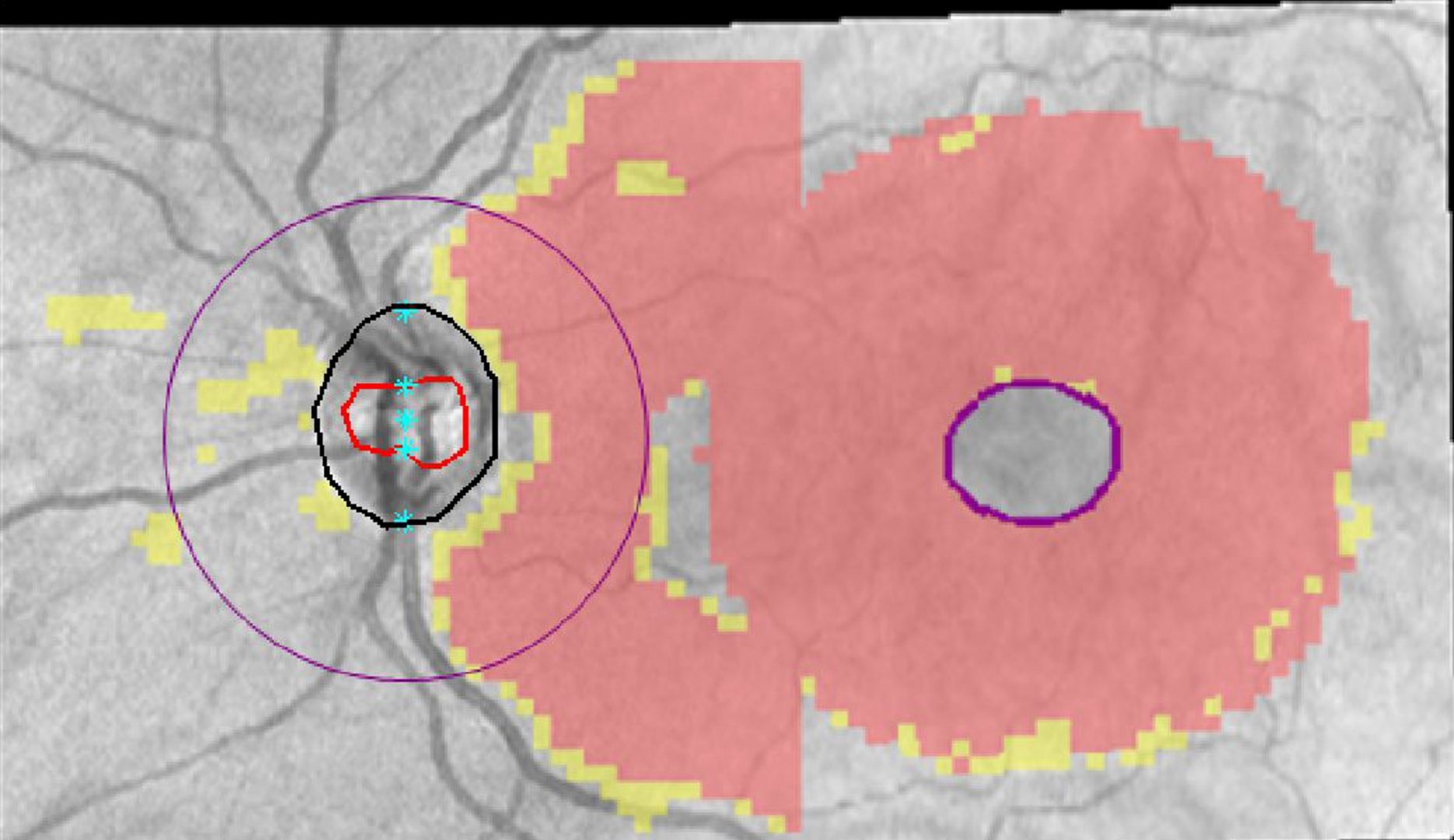
The vertical and horizontal tomograms identify the edge of the cup (red dot) and edge of the disc (black dot). Identification is based on Bruch's membrane opening rather than the visible disc margins. Mis-identification of these features can occur due to peripapillary atrophy.
RNFL Analysis
-
RNFL thickness map
The RNFL thickness map (also referred to as a heat map) shows the RNFL thickness measurements using a colour pattern. This map is not based on comparisons to the normative database. Cool colours (blue) represent thinner values and warm colours (yellow or red) represent thicker values.
-
RNFL Deviation Map
The RNFL deviation map provides a statistical comparison against the normative database overlaid on the OCT fundus image. Any yellow or red pixel colours indicate that the average thickness falls within the corresponding distribution percentiles. Any region without yellow or red pixels indicate that thickness values fall within the normal limits.
-
Global Parameters
The global parameters give numerical measurements for the following:
1. Rim area: This is the surface area of the disc, excluding the cup. The bigger the size of the cup, the smaller the rim area.
2. CD ratio: This parameter should be viewed with caution as it is often not accurate or repeatable due to delineation errors of the cup/disc margin.
3. Cup volume: This measurement is taken from the OCT b-scans. Increased cupping is associated with a higher cup volume.
4. Disc area: The edge of the disc is defined differently by different OCT instruments, however it is typically the termination of the RPE/Bruch's membrane. This measurement can be affected by delineation errors. The disc area is normally between 1.7 and 2 square millimeters (Knight et al.).Most of these parameters can be assessed through our funduscopic examination of the optic nerve and therefore may not be commonly used in clinical practice.
-
RNFL Thickness (TSNIT) curve
The TSNIT curve (TSNIT stands for temporal, superior, nasal, inferior, temporal) represents the RNFL thickness calculated along 256 radial A-scans evenly spaced around the optic nerve head. This TSNIT curve is superimposed on a white-green-yellow-red background based on the normative database.
The TSNIT curve is useful in visualising RNFL loss and for comparing symmetry between the two eyes.
-
RNFL Quadrant and Clock Hour Analysis
The quadrant and clock hour analysis utilise the same data as the TSNIT curve (256 radial A-scans evenly spaced around the optic nerve head). It averages the RNFL thickness within the given clock hour or quadrant to produce a numerical value, allowing comparison of raw data. RNFL thickness in each clock hour or quadrant is compared to the normative distribution with areas of thinning flagged as yellow or red.
As these values represent an average, small RNFL defects can be masked, particularly if the area of thinning is adjacent to an area increased thickness.
-
Symmetry Analysis
Typically the RNFL profile is relatively symmetrical between the two eyes in a healthy patient. Comparison of RNFL thickness maps, TSNIT curves and the RNFL quadrant/ clock hour thickness can help identify areas of thinning. It is important to not rely on the colour codes only which may suggest RNFL thickness is within normal limits and 'green'. The presence of 'green disease' can cause misdiagnosis and is covered later in this section.
Physiological Variations
-
Split bundle
A split-bundle refers to an atypical arrangement of the superior retinal nerve fibres. In this presentation, the nerve fibres that would typically be positioned superiorly have been laterally displaced. or "split" into two parts.
In this physiological variation, the RNFL heat map will show a symmetrically divided RNFL appearance while the deviation map may flag RNFL thinning in-between these two bundles. This s not a true thinning, rather the software is identifying that the RNFL is thinner than the normative age-matched thickness in that area. On either side of this superior split, the RNFL is typically thicker than the normative distribution, however thickening is not flagged on the deviation map so this is harder to appreciate.
A split-bundle defect is associated with a "double hump" superiorly on the TSNIT curve, reflecting the increased thickness supero-temporal and supero-nasally.
-
Temporal RNFL shift
A temporal RNFL shift is another physiological variation associated with redistribution of the RNFL. In this situation, the superior and inferior RNFL are shifted temporally. As a result the deviation map may flag superior and inferior RNFL loss which can resemble glaucomatous loss.
The TSNIT curve will show a temporal displacement of the superior and inferior RNFL bundle.
Ganglion Cell Analysis
-
GCA thickness map
The GCA measures the thickness of the ganglion cell-inner plexiform layer (GCIPL) which is located directly underneath the RNFL on an OCT line scan. The GCA thickness map (also referred to as a heat map) shows the relative thickness of the GCIPL. This map is not based on a normative comparison, but rather shows thickness values only.
-
GCA Deviation Map
The deviation map is produced using pixel by pixel analysis of the GCIPL thickness and compare this with the normative database.
-
Global Parameters
These parameters provide average and minimum GCIPL thickness. In a healthy patient, these metrics will be similar between the two eyes while in disease, the numbers may fall outside normative parameters or be asymmetric.
GCL+IPL thicknesses flagged green are within normative limits while those flagged yellow and red indicate possible loss.
-
GCA Sector Analysis
The sector analysis allows numerical comparison of the GCIPL thickness in different anatomical locations. Similar to the RNFL quadrant analysis, this metric averages the GCIPL thickness measurements for a given sector. Sectors are typically similar in thickness between the two eyes when comparing equivalent sectors (for example when comparing temporal measurements in the right with temporal measurements in the left.
Green Disease
-
Overview
In OCT analysis, green disease is a term used to describe a situation where disease/damage is present but the OCT software calculates that the RNFL or GCIPL thickness is within the normative distribution so flags this "green". This can lead to the practitioner misdiagnosing a glaucomatous eye as normal.
Some potential causes of green disease are incorrect segmentation, subtle RNFL loss, macular pathology and a physiologically thicker RNFL prior to disease-induced thinning.
To detect green disease, it is important to check segmentation, but also to look at the raw data. Typically you expect a high degree of inter-eye symmetry. Areas of asymmetry, particularly superotemporally and inferotemporally, between the eyes should raise suspicion even if the thickness values are 'green'. This can be done by assessing the TSNIT curve or comparing clock hour or quadrant thicknesses. At this point it is important to note that when making these comparisons, you should compare like with like - i.e. compare temporal clock hours in the right with temporal clock hours in the left.
There is some test-retest variability in RNFL thicknesses, so a differential between the two eyes is only considered significant over 9-12µm (depending on the instrument used). Asymmetry above this level is considered suspicious for glaucomatous damage (Budenz et al. 2008)
-
Case 1
A 65 year old female with a family history of glaucoma in both parents. Intraocular pressures were 22mmHg in the right eye and 24mmHg in the left eye. Central corneal thicknesses were 516µm in each eye.
-
Case 2
A 49 year old Asian female with moderate myopia, good general health and no family history of glaucoma. She has intraocular pressures of 19mmHg in each eye. Central corneal thickness are 576µm right eye and 583µm left eye.
Red Disease
-
Overview
Red disease is a term used to describe a false positive diagnosis where the OCT instrument flags an area of RNFL loss, however there is no disease process present.
Common causes of red disease include split bundle configurations, temporal RNFL shift (both described above) and imaging artefacts such as media opacities.
-
Case 1
A 28 year old female with moderately high myopia and intraocular pressures of 11mmHg in each eye in the context of average pachymetry measurements (545µm in each eye). She has no family history of glaucoma and takes no medications. Gonioscopic examination revealed angles open to the ciliary body band in all quadrants and no signs of secondary glaucoma. 24-2 threshold visual fields were unremarkable in both eyes.
-
Case 2
A 20 year old Caucasian female with moderate myopia and intraocular pressures of 17mmHg in each eye. Gonioscopy showed angles open to the ciliary body band in all quadrants and no signs of secondary glaucoma. 24-2 threshold visual fields were unremarkable in both eyes.
References
Bayer A, Akman A. Artifacts and Anatomic Variations in Optical Coherence Tomography. Turk J Ophthalmol. 2020;50(2):99-106.
Budenz DL. Symmetry between the right and left eyes of the normal retinal nerve fiber layer measured with optical coherence tomography (an AOS thesis). Trans Am Ophthalmol Soc. 2008;106:252-275.
Chen JJ, Kardon RH. Avoiding Clinical Misinterpretation and Artifacts of Optical Coherence Tomography Analysis of the Optic Nerve, Retinal Nerve Fiber Layer, and Ganglion Cell Layer. J Neuroophthalmol. 2016;36(4):417-438.
Sayed MS, Margolis M, Lee RK. Green disease in optical coherence tomography diagnosis of glaucoma. Curr Opin Ophthalmol. 2017 Mar;28(2):139-153.
Tai ELM, Ling JL, Gan EH, Adil H, Wan-Hazabbah WH. Comparison of peripapillary retinal nerve fiber layer thickness between myopia severity groups and controls. Int J Ophthalmol. 2018;11(2):274-278.